Portfolio construction techniques based on predicted risk, without expected returns, have become quite popular within the last couple of years. Especially on Seeking Alpha, great articles have been published by fellow contributors, covering the full range of modern portfolio theory and other different kind of tactical asset allocation concepts.
Our research paper, published and awarded as Editor’s Pick on Seeking Alpha, analyzes and compares ten modern portfolio construction techniques by applying an advanced Monte Carlo Simulation. This enables an unbiased view of the pros and cons of each single portfolio construction technique.
However, most of those published articles are based on back testing, whereas limited historical data as well as highly unlikely similar future performances of certain asset classes (e.g. the 30-year bull market in bonds or the very nice trend structure of equities between 2000 and 2010) are making an evaluation or comparisons of different kind of portfolio construction techniques quite difficult. Of course, this issue has led to many questions by fellow readers, how a certain portfolio would have performed, if there had been a huge decline in the bond market or if other tail-events would have happened. Since many of these questions have not been answered yet, we would like to analyze and compare ten popular portfolio construction techniques by applying an advanced Monte Carlo simulation to avoid using historical data. Therefore, we will be able to get an unbiased view of the pros and cons of each single portfolio construction technique.
In terms of asset selection, we are reviewing the following concepts:
As already mentioned above, we are using a Monte Carlo simulation, to generate 300 years of daily data. In general, a Monte Carlo simulation performs any kind of analysis by building samples of possible results by substituting a range of values (a probability distribution) for any factor that has inherent uncertainty. It then calculates results over and over, each time using a different set of random values from the probability function. In other words, it is possible to simulate umpteen years of data, which have more or less the same risk characteristics as the desired underlying asset classes.
In our example, we will use a multivariate normal distribution, which is fitted with certain parameters (return- and correlation estimates) in order to describe the random behavior (market riskiness) of asset returns. Worth mentioning is the fact that the input parameters are just a point of reference since the multivariate normal distribution will randomly generate values within the normal standard distribution. However, when it comes to simulations, the results should be seen as an additional source of information rather than an all explaining framework. For that reason, all the results should be treated with caution and should just be seen as another mosaic stone in quantitative finance.
According to a Bridgewater research paper, betas (asset classes) have had, and are expected to have, ratios of excess returns to excess risks (Sharpe Ratios) of about 0.2 to 0.3. That is because:
“there needs to be some extra return to compensate investors for excess risk (so this ratio should be positive), but this ratio cannot be very extremely positive because that would make these investments attract substantial amounts of capital that would bid up their prices and lower their expected return.”
Therefore, we have used an average return estimation for each asset class, which produces Sharpe Ratios of 0.2 to 0.3, whereas the risk free rate is 1.5 percent. Furthermore, we have used the historical variance-/covariance matrix from 1980 until 2013 for the iShares Core S&P 500 ETF (IVV), the iShares Core Total U.S. Bond Market ETF (AGG), the UBS ETRACS DJ-UBS Commodity Index Total Return ETN (DJCI) and the SPDR Gold Shares (GLD), as reference points for the underlying correlation assumptions.
Summary statistics, drawdowns as well as a performance chart (logarithmic scale) for the four simulated asset classes are given below. As you can see, the Sharpe Ratios for the underlying securities are almost equal, since they are ranging between 0.17 and 0.23, which can be seen as a quite conservative outcome. More importantly, with a maximum loss of 87 percent, equities have faced the highest decline in the past, followed by gold, commodities and bonds. Another interesting fact is the decline of bonds by almost 40 percent, a situation which we have not seen in the last couple of decades. Therefore, it will be quite interesting to see, how bond-heavy portfolio construction techniques will perform under such conditions. However, the overall key statistics are looking quite reasonable and therefore the simulated time series can be seen as a quite good proxy for evaluating the above mentioned portfolio concepts.
Table 1: Key Statistics ETFs – Performance Ratios [1700-2000]
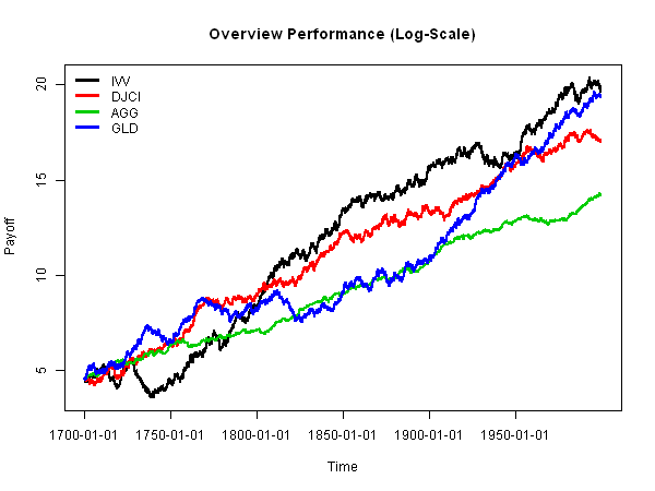
Chart 1: Performance Chart ETFs – Overview Performance
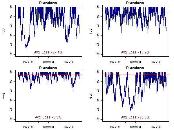
Chart 2: Drawdowns ETFs
In our example, there is no allowance for transaction costs or brokerage fees. In order to minimize transaction costs, we rebalance the portfolio on a monthly basis, whereas 1-day slippage is included. In addition, we have determined the weights for all portfolio concepts on a monthly basis. Worth mentioning is the fact that we are using a rolling variance/co-variance matrix to determine the weights for all risk-based concepts, as correlations among asset classes are not stable over time.
The simulation results are summarized in the table below. The most favorable portfolio in terms of performance is the Minimum Correlation Portfolio (“MCP”), with an annualized return of 5.87 percent, followed by the Momentum Based Portfolio (“MBP”) with 5.55 percent and the Most Diversified Portfolio (“MDP”) with 5.3 percent. With slightly more than 4 percent, the IVY Portfolio (“IVY”) is delivering the lowest compound annual growth rate, followed by the Classical Balanced Portfolio (“CBP”), with an average return of 4.07 percent a year.
Table 2: Key Statistics Portfolios
However, return is just telling one side of the story. For that reason, the Sharpe Ratio is a better measure to examine the risk/reward ratio. The Most Diversified Portfolio has the highest Sharpe Ratio, followed by the Permanent Portfolio (“PEP”) and the Risk Parity Portfolio (“RPP”).
This result is strongly in-line with the theoretical background, as there should be no other portfolio combination, which can achieve a higher risk-/return ratio than the Most Diversified Portfolio (“MDP”).
In general, 5 out of 10 portfolio concepts had Sharpe Ratios above 0.5. Moreover, the Classic Balanced Portfolio (“CBP”), as well as all timing based portfolio concepts (“MBP,” “IVY”) are delivering the lowest Sharpe Ratios.
A quite good reason for that outcome is the fact that those portfolios are not as well diversified as their peers and therefore their overall portfolio volatility is either too high (“CBP” and the “MBP”) or their average return is too low (“IVY”).
In terms of risk, the Global Minimum Variance Portfolio (“GMV”) has of course the lowest portfolio volatility, whereas the Momentum Based Portfolio (“MBP”) and the Minimum Correlation Portfolio (“MCP”) are having by far the highest ones.
To evaluate the absolute return character of each portfolio construction technique, we will have a closer look on the ability of each concept to generate absolute returns on a yearly basis as well as on the maximal- and average drawdown statistics of those portfolios.
Within almost 300 years of data, the Most Diversified Portfolio (“MDP”) as well as the Minimum Tail Depended Portfolio (“MTP”) had only 24 negative years, followed by the Permanent Portfolio (“PEP”) and the Risk Parity Portfolio (“RPP”) with 25 years of negative returns. The Global Minimum Variance Portfolio (“GMV”) failed to deliver positive returns in 27 years, whereas all other portfolio concepts had negative returns in 30 (“MBP”) years or above (“IVY”, “MCP” and the “CBP”).
The IVY Portfolio (“IVY”) as well as the Global Minimum Variance (“GMV”) had the lowest maximal drawdown, whereas the Minimum Correlation Portfolio (“MCP”) as well as the Momentum Based Portfolio (“MBP”) had by far the highest ones. Another highly interesting fact is that the largest drawdown of most portfolios did not occur within the same time period in which their underlying asset classes suffered the most (see table below).
Table 3: Largest Drawdowns ETFs & Portfolios
Especially, the Risk Parity Portfolio (“RPP”) and the Most Diversified Portfolio (“MDP”) were holding up quite well, during that time the bond market crashed, while the Global Minimum Variance Portfolio (“GMV”) was hurt the most! This outcome is not surprising at all, since the Global Minimum Variance Portfolio (“GMV”) is heavily weighted in bonds and in addition, this concept does not utilize all benefits from diversification.
As already mentioned in other articles, as long as the correlations within the underlying asset classes remain low, the Risk Parity Portfolio (“RPP”) as well as the Most Diversified Portfolio (“MDP”) won’t be hurt too much, in times of rising interest rates, although they are also heavily weighted in bonds. This is mainly due to the effect, that other asset classes are offsetting the negative performance of bonds.
In general, prices do not go down to zero overnight and therefore it still makes sense to keep a declining asset class within the portfolio, due to their diversification benefits.
For example, if there is a normal correction within an ongoing equity bull market, bonds still tend to rise although they might be in a longer lasting down-trend. This will lead to smoother returns and less drawdowns, which is one of the main strengths of those new portfolio construction concepts.
Furthermore, we can see that apart from the Minimum Correlation Portfolio (“MCP”), the Classic Balanced Portfolio (“CBP”) and the Global Minimum Variance (“GMV”), all other concepts had their worst performance more or less during the same time period.
Since the historical maximum drawdown is just representing a single tail event in the past, the average drawdowns are much more accurate to evaluate the absolute return character of each construction technique.
Below, we have charted all drawdowns as well as the average loss of each portfolio. There we can see that the Permanent Portfolio (“PEP”) as well as the Most Diversified Portfolio (“MDP”) had the lowest drawdowns on average, whereas the Minimum Correlation Portfolio (“MCP”), the Classic Balanced Portfolio (“CBP”) as well as the Momentum Based Portfolio (“MBP”) had the highest ones.
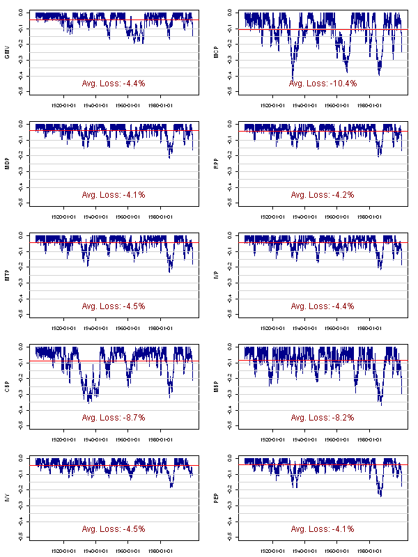
Chart 3: Drawdowns Portfolios
To make things more clear, we have ranked the portfolios with numbers ranging from 10 to 1, where 10 represents the most favorable result. Furthermore, we have averaged all scores, to get a total score for each portfolio. There we can see that the Most Diversified Portfolio (“MDP”) has got the highest average score and is therefore representing a good mixture between performance and risk. The Risk Parity Portfolio (“RPP”) is on the second place, with a score of 7.5, followed by the Permanent Portfolio (“PEP”) and Global Minimum Variance Portfolio (“GMV”). However, with 2 points, the Classic Balanced Portfolio (“CBP”) has received the lowest score among all evaluated portfolio construction concepts, followed by the Minimum Correlation Portfolio (“MCP”) and the Momentum Based Portfolio (“MBP”)!
Table 3: Ranking Portfolios
Basically, all portfolio construction techniques are delivering higher Sharpe Ratios than their underlying asset classes, which is just another proof of the overall diversification concept.
The Global Minimum Variance Portfolio (“GMV”) is still doing a good job although it will definitely get hurt the most if we see rising interest rates in the future. As already mentioned in our previous articles, a huge decline in the bond market will not automatically lead to such catastrophic scenarios for the Risk Parity Portfolio (“RPP”) or the Most Diversified Portfolio (“MDP”), as some fellow readers might have thought.
In contrast, the Inverse Volatility Portfolio (“IVP”), which is often mixed-up with the risk parity approach, is underperforming its bigger brother (“RPP”) in terms of its overall score. If we focus on portfolios that are based on timing rather than portfolio construction, we can see that the typical late-in, late-out effect of those concepts will mostly lead to increased volatility or low returns, which is of course affecting their Sharpe Ratios as well as other risk/performance based ratios.
The Minimum Correlation Portfolio (“MCP”) does not utilize all the benefits, which can be achieved by diversification, and if we have a look at this specific weighting algorithm, we do not really see any big advantage over other concepts.
The Minimum Tail Dependent Portfolio (“MTP”) has shown quite robust results and given a Sharpe Ratio above 0.5, it is definitely worth an investment. However, as this optimization concept needs a lot of estimates (via copula), we think it might be a bit challenging for common investors to understand the rationale behind it.
In contrast, the Permanent Portfolio (“PEP”) defended its reputation, to be a good and simple investment concept as it has delivered the third highest Sharpe Ratio and the third highest overall score.
Furthermore, we can say that the Classic Balanced Portfolio (“CBP”) is by far the worst concept, followed by the Momentum Based Portfolio (“MBP”), whereas the Most Diversified Portfolio (“MDP”) has shown once again that diversification pays off the most, as it is the only free lunch an investor has!
Author: Robert C. Koch
Note: This research publication was published and awarded as Editor’s Pick on Seeking Alpha in September 2013.
Start your journey towards informed and strategic investment decisions. With WallStreetCourier, you have the tools and insights to navigate market trends confidently. Join us today and transform your approach to trend following.
You are currently viewing a placeholder content from X. To access the actual content, click the button below. Please note that doing so will share data with third-party providers.
More Information